Probability distribution: Difference between revisions
→With finite support: That does not make any sense (what "input"?). |
wrote intro (see talk) |
||
| Line 1: | Line 1: | ||
A '''probability distribution''' describes the ''values'' and ''[[probabilities]]'' that a [[random event]] can take. The values must cover all of the possible outcomes of the event, while the total probabilities must [[sum]] to exactly 1, or 100%. For example, a single coin flip can take values ''Heads'' or ''Tails'' with a probability of exactly 1/2 for each: This set of two values and two probabilities make up the probability distribution of the single coin flipping event. This distribution is called a ''[[discrete probability distribution|discrete distribution]]'' because there are an exact, countable number of outcomes to the event. |
|||
A ''[[continuous probability distribution|continuous distribution]]'' describes events over a continuous range, where the probability of a specific outcome is zero. For example, a dart thrown at a dartboard has essentially zero probability of landing at a specific point, since a point is [[infinitesimal|vanishingly small]], but it has some probability of landing within a given area. The probability of landing within the small area of the bullseye would (hopefully) be greater than landing on an equivalent area elsewhere on the board. A smooth function that describes the probability of landing anywhere on the dartboard is the probability distribution of the dart throwing event. The [[integral]] of the [[probability density function]] (pdf) over the entire area of the dartboard (and, perhaps, the wall surrounding it) must be equal to 1, since each dart must land somewhere. |
|||
The concept of the probability distribution underlies the mathematical discipline of [[probability theory]], and the science of [[statistics]]. There is spread or variability in almost any value that can be measured in a population (e.g. height of people, durability of a metal, etc.); almost all measurements is made with some [[measurement error|error]]; in [[physics]] many processes, from the properties of gases to the the [[quantum mechanical]] description of [[fundamental particles]] is probabilistic. For these and many other reasons, simple [[numbers]] are often inadequate for describing a quantity; whereas probability distributions are often more appropriate models. There are, however, considerable mathematical complications in manipulating probability distributions, since most standard [[arithmetic]] and [[algebraic]] manipulations cannot be applied to distributions in the same was as to numeric quantities. |
|||
= Rigorous definitions = |
|||
In [[probability theory]], every [[random variable]] may be attributed to a function defined on a state space equipped with a '''probability distribution''' that assigns a [[probability]] to every [[subset]] (more precisely every measurable subset) of its [[probability space|state space]] in such a way that the [[probability axioms]] are satisfied. That is, probability distributions are [[probability measure]]s defined over a state space instead of the sample space. A random variable then defines a probability measure on the sample space by assigning a subset of the sample space the probability of its inverse image in the state space. In other words the probability distribution of a random variable is the [[push forward measure]] of the probability distribution on the state space. |
In [[probability theory]], every [[random variable]] may be attributed to a function defined on a state space equipped with a '''probability distribution''' that assigns a [[probability]] to every [[subset]] (more precisely every measurable subset) of its [[probability space|state space]] in such a way that the [[probability axioms]] are satisfied. That is, probability distributions are [[probability measure]]s defined over a state space instead of the sample space. A random variable then defines a probability measure on the sample space by assigning a subset of the sample space the probability of its inverse image in the state space. In other words the probability distribution of a random variable is the [[push forward measure]] of the probability distribution on the state space. |
||
| Line 38: | Line 46: | ||
A '''discrete random variable''' is a random variable whose probability distribution is discrete. Similarly, a '''continuous random variable''' is a random variable whose probability distribution is continuous. |
A '''discrete random variable''' is a random variable whose probability distribution is discrete. Similarly, a '''continuous random variable''' is a random variable whose probability distribution is continuous. |
||
= List of important probability distributions = |
|||
Certain random variables occur very often in probability theory, in some cases due to their application to many natural and physical processes, and in some cases due to theoretical reasons such as the [[central limit theorem]], the [[Poisson limit theorem]], or properties such as [[memorylessness]] or other [[characterization (mathematics)|characterizations]]. Their distributions therefore have gained ''special importance'' in probability theory. |
Certain random variables occur very often in probability theory, in some cases due to their application to many natural and physical processes, and in some cases due to theoretical reasons such as the [[central limit theorem]], the [[Poisson limit theorem]], or properties such as [[memorylessness]] or other [[characterization (mathematics)|characterizations]]. Their distributions therefore have gained ''special importance'' in probability theory. |
||
==Discrete distributions== |
|||
===With finite support=== |
|||
*The [[Bernoulli distribution]], which takes value 1 with probability ''p'' and value 0 with probability ''q'' = 1 − ''p''. |
*The [[Bernoulli distribution]], which takes value 1 with probability ''p'' and value 0 with probability ''q'' = 1 − ''p''. |
||
| Line 54: | Line 62: | ||
* The [[Zipf-Mandelbrot law]] is a discrete power law distribution which is a generalization of the [[Zipf distribution]]. |
* The [[Zipf-Mandelbrot law]] is a discrete power law distribution which is a generalization of the [[Zipf distribution]]. |
||
===With infinite support=== |
|||
* The [[Boltzmann distribution]], a discrete distribution important in [[statistical physics]] which describes the probabilities of the various discrete energy levels of a system in [[thermal equilibrium]]. It has a continuous analogue. Special cases include: |
* The [[Boltzmann distribution]], a discrete distribution important in [[statistical physics]] which describes the probabilities of the various discrete energy levels of a system in [[thermal equilibrium]]. It has a continuous analogue. Special cases include: |
||
| Line 72: | Line 80: | ||
* The [[zeta distribution]] has uses in applied statistics and statistical mechanics, and perhaps may be of interest to number theorists. It is the [[Zipf distribution]] for an infinite number of elements. |
* The [[zeta distribution]] has uses in applied statistics and statistical mechanics, and perhaps may be of interest to number theorists. It is the [[Zipf distribution]] for an infinite number of elements. |
||
==Continuous distributions== |
|||
===Supported on a bounded interval=== |
|||
[[Image:Beta distribution pdf.png|thumb|150px|[[Beta distribution]]]] |
[[Image:Beta distribution pdf.png|thumb|150px|[[Beta distribution]]]] |
||
* The [[Beta distribution]] on [0,1], of which the uniform distribution is a special case, and which is useful in estimating success probabilities. |
* The [[Beta distribution]] on [0,1], of which the uniform distribution is a special case, and which is useful in estimating success probabilities. |
||
| Line 90: | Line 98: | ||
*The [[Wigner semicircle distribution]] is important in the theory of [[random matrices]]. |
*The [[Wigner semicircle distribution]] is important in the theory of [[random matrices]]. |
||
===Supported on semi-infinite intervals, usually <nowiki>[0,∞)</nowiki>=== |
|||
[[Image:Chi-square distributionPDF.png|thumb|150px|[[chi-square distribution]]]] |
[[Image:Chi-square distributionPDF.png|thumb|150px|[[chi-square distribution]]]] |
||
* The [[chi distribution]] |
* The [[chi distribution]] |
||
| Line 121: | Line 129: | ||
* The [[Weibull distribution]], of which the exponential distribution is a special case, is used to model the lifetime of technical devices. |
* The [[Weibull distribution]], of which the exponential distribution is a special case, is used to model the lifetime of technical devices. |
||
===Supported on the whole real line=== |
|||
[[Image:Cauchy distribution pdf.png|150px|thumb|[[Cauchy distribution]]]] |
[[Image:Cauchy distribution pdf.png|150px|thumb|[[Cauchy distribution]]]] |
||
[[Image:Laplace distribution pdf.png|150px|thumb|[[Laplace distribution]]]] |
[[Image:Laplace distribution pdf.png|150px|thumb|[[Laplace distribution]]]] |
||
| Line 144: | Line 152: | ||
* The [[Voigt profile|Voigt distribution]], or Voigt profile, is the convolution of a [[normal distribution]] and a [[Cauchy distribution]]. It is found in spectroscopy when [[spectral line]] profiles are broadened by a mixture of [[Lorentzian function|Lorentzian]] and [[Doppler profile|Doppler]] broadening mechanisms. |
* The [[Voigt profile|Voigt distribution]], or Voigt profile, is the convolution of a [[normal distribution]] and a [[Cauchy distribution]]. It is found in spectroscopy when [[spectral line]] profiles are broadened by a mixture of [[Lorentzian function|Lorentzian]] and [[Doppler profile|Doppler]] broadening mechanisms. |
||
==Joint distributions== |
|||
For any set of [[Statistical independence|independent]] random variables the [[probability density function]] of their [[joint distribution]] is the product of their individual density functions. |
For any set of [[Statistical independence|independent]] random variables the [[probability density function]] of their [[joint distribution]] is the product of their individual density functions. |
||
===Two or more random variables on the same sample space=== |
|||
* [[Dirichlet distribution]], a generalization of the [[beta distribution]]. |
* [[Dirichlet distribution]], a generalization of the [[beta distribution]]. |
||
| Line 156: | Line 164: | ||
* [[multivariate normal distribution]], a generalization of the [[normal distribution]]. |
* [[multivariate normal distribution]], a generalization of the [[normal distribution]]. |
||
===Matrix-valued distributions=== |
|||
*[[Wishart distribution]] |
*[[Wishart distribution]] |
||
| Line 163: | Line 171: | ||
*[[Hotelling's T-square distribution]] |
*[[Hotelling's T-square distribution]] |
||
==Miscellaneous distributions== |
|||
* The [[Cantor distribution]] |
* The [[Cantor distribution]] |
||
| Line 169: | Line 177: | ||
* [[Truncated distribution]] |
* [[Truncated distribution]] |
||
=Demonstrations and activities= |
|||
The [[SOCR]] resource provides web-based tools (applets) for [http://www.socr.ucla.edu/htmls/SOCR_Modeler.html sampling from] and [http://www.socr.ucla.edu/htmls/SOCR_Distributions.html interacting with] many of these discrete and continuous distributions. Also, a number of [http://wiki.stat.ucla.edu/socr/index.php/SOCR_EduMaterials_DistributionsActivities distribution-specific activities] are provided that demonstrate the utilization of general probability distributions. |
The [[SOCR]] resource provides web-based tools (applets) for [http://www.socr.ucla.edu/htmls/SOCR_Modeler.html sampling from] and [http://www.socr.ucla.edu/htmls/SOCR_Distributions.html interacting with] many of these discrete and continuous distributions. Also, a number of [http://wiki.stat.ucla.edu/socr/index.php/SOCR_EduMaterials_DistributionsActivities distribution-specific activities] are provided that demonstrate the utilization of general probability distributions. |
||
= See also = |
|||
*[[copula (statistics)]] |
*[[copula (statistics)]] |
||
| Line 186: | Line 194: | ||
{{Statistics}} |
{{Statistics}} |
||
=External links= |
|||
{{commons|Probability distribution|Probability distribution}} |
{{commons|Probability distribution|Probability distribution}} |
||
Revision as of 02:32, 29 November 2007
A probability distribution describes the values and probabilities that a random event can take. The values must cover all of the possible outcomes of the event, while the total probabilities must sum to exactly 1, or 100%. For example, a single coin flip can take values Heads or Tails with a probability of exactly 1/2 for each: This set of two values and two probabilities make up the probability distribution of the single coin flipping event. This distribution is called a discrete distribution because there are an exact, countable number of outcomes to the event.
A continuous distribution describes events over a continuous range, where the probability of a specific outcome is zero. For example, a dart thrown at a dartboard has essentially zero probability of landing at a specific point, since a point is vanishingly small, but it has some probability of landing within a given area. The probability of landing within the small area of the bullseye would (hopefully) be greater than landing on an equivalent area elsewhere on the board. A smooth function that describes the probability of landing anywhere on the dartboard is the probability distribution of the dart throwing event. The integral of the probability density function (pdf) over the entire area of the dartboard (and, perhaps, the wall surrounding it) must be equal to 1, since each dart must land somewhere.
The concept of the probability distribution underlies the mathematical discipline of probability theory, and the science of statistics. There is spread or variability in almost any value that can be measured in a population (e.g. height of people, durability of a metal, etc.); almost all measurements is made with some error; in physics many processes, from the properties of gases to the the quantum mechanical description of fundamental particles is probabilistic. For these and many other reasons, simple numbers are often inadequate for describing a quantity; whereas probability distributions are often more appropriate models. There are, however, considerable mathematical complications in manipulating probability distributions, since most standard arithmetic and algebraic manipulations cannot be applied to distributions in the same was as to numeric quantities.
Rigorous definitions
In probability theory, every random variable may be attributed to a function defined on a state space equipped with a probability distribution that assigns a probability to every subset (more precisely every measurable subset) of its state space in such a way that the probability axioms are satisfied. That is, probability distributions are probability measures defined over a state space instead of the sample space. A random variable then defines a probability measure on the sample space by assigning a subset of the sample space the probability of its inverse image in the state space. In other words the probability distribution of a random variable is the push forward measure of the probability distribution on the state space.
Probability distributions of real-valued random variables
Because a probability distribution Pr on the real line is determined by the probability of being in a half-open interval Pr(a, b], the probability distribution of a real-valued random variable X is completely characterized by its cumulative distribution function:
Discrete probability distribution
A probability distribution is called discrete if its cumulative distribution function only increases in jumps.
The set of all values that a discrete random variable can assume with non-zero probability is either finite or countably infinite because the sum of uncountably many positive real numbers (which is the smallest upper bound of the set of all finite partial sums) always diverges to infinity. Typically, the set of possible values is topologically discrete in the sense that all its points are isolated points. But, there are discrete random variables for which this countable set is dense on the real line.
Discrete distributions are characterized by a probability mass function, such that
Continuous probability distribution
By one convention, a probability distribution is called continuous if its cumulative distribution function is continuous, which means that it belongs to a random variable X for which Pr[ X = x ] = 0 for all x in R.
Another convention reserves the term continuous probability distribution for absolutely continuous distributions. These distributions can be characterized by a probability density function: a non-negative Lebesgue integrable function defined on the real numbers such that
Discrete distributions and some continuous distributions (like the devil's staircase) do not admit such a density.
Terminology
The support of a distribution is the smallest closed set whose complement has probability zero.
The probability distribution of the sum of two independent random variables is the convolution of each of their distributions.
The probability distribution of the difference of two random variables is the cross-correlation of each of their distributions.
A discrete random variable is a random variable whose probability distribution is discrete. Similarly, a continuous random variable is a random variable whose probability distribution is continuous.
List of important probability distributions
Certain random variables occur very often in probability theory, in some cases due to their application to many natural and physical processes, and in some cases due to theoretical reasons such as the central limit theorem, the Poisson limit theorem, or properties such as memorylessness or other characterizations. Their distributions therefore have gained special importance in probability theory.
Discrete distributions
With finite support
- The Bernoulli distribution, which takes value 1 with probability p and value 0 with probability q = 1 − p.
- The Rademacher distribution, which takes value 1 with probability 1/2 and value −1 with probability 1/2.
- The binomial distribution describes the number of successes in a series of independent Yes/No experiments.
- The degenerate distribution at x0, where X is certain to take the value x0. This does not look random, but it satisfies the definition of random variable. It is useful because it puts deterministic variables and random variables in the same formalism.
- The discrete uniform distribution, where all elements of a finite set are equally likely. This is supposed to be the distribution of a balanced coin, an unbiased die, a casino roulette or a well-shuffled deck. Also, one can use measurements of quantum states to generate uniform random variables. All these are "physical" or "mechanical" devices, subject to design flaws or perturbations, so the uniform distribution is only an approximation of their behaviour. In digital computers, pseudo-random number generators are used to produce a statistically random discrete uniform distribution.
- The hypergeometric distribution, which describes the number of successes in the first m of a series of n Yes/No experiments, if the total number of successes is known.
- Zipf's law or the Zipf distribution. A discrete power-law distribution, the most famous example of which is the description of the frequency of words in the English language.
- The Zipf-Mandelbrot law is a discrete power law distribution which is a generalization of the Zipf distribution.
With infinite support
- The Boltzmann distribution, a discrete distribution important in statistical physics which describes the probabilities of the various discrete energy levels of a system in thermal equilibrium. It has a continuous analogue. Special cases include:
- The geometric distribution, a discrete distribution which describes the number of attempts needed to get the first success in a series of independent Yes/No experiments.

- The logarithmic (series) distribution
- The negative binomial distribution, a generalization of the geometric distribution to the nth success
- The parabolic fractal distribution
- The Poisson distribution, which describes a very large number of individually unlikely events that happen in a certain time interval.

- The Skellam distribution, the distribution of the difference between two independent Poisson-distributed random variables
- The Yule-Simon distribution
- The zeta distribution has uses in applied statistics and statistical mechanics, and perhaps may be of interest to number theorists. It is the Zipf distribution for an infinite number of elements.
Continuous distributions
Supported on a bounded interval

- The Beta distribution on [0,1], of which the uniform distribution is a special case, and which is useful in estimating success probabilities.

- The continuous uniform distribution on [a,b], where all points in a finite interval are equally likely.
- The rectangular distribution is a uniform distribution on [-1/2,1/2].
- The Dirac delta function although not strictly a function, is a limiting form of many continuous probability functions. It represents a discrete probability distribution concentrated at 0 — a degenerate distribution — but the notation treats it as if it were a continuous distribution.
- The Kent distribution on the three-dimensional sphere
- The Kumaraswamy distribution is as versatile as the Beta distribution but has simple closed forms for both the cdf and the pdf.
- The logarithmic distribution (continuous)
- The triangular distribution on [a, b], a special case of which is the distribution of the sum of two uniformly distributed random variables (the convolution of two uniform distributions).
- The truncated normal distribution on [a, b]
- The U-quadratic distribution on [a, b]
- The von Mises distribution on the circle
- The von Mises-Fisher distribution on the N-dimensional sphere has the von Mises distribution as a special case.
- The Wigner semicircle distribution is important in the theory of random matrices.
Supported on semi-infinite intervals, usually [0,∞)

- The chi distribution
- The noncentral chi distribution
- The chi-square distribution, which is the sum of the squares of n independent Gaussian random variables. It is a special case of the Gamma distribution, and it is used in goodness-of-fit tests in statistics.
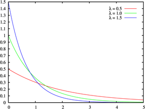
- The exponential distribution, which describes the time between consecutive rare random events in a process with no memory.
- The F-distribution, which is the distribution of the ratio of two (normalized) chi-square distributed random variables, used in the analysis of variance. (Called the beta prime distribution when it is the ratio of two chi-square variates which are not normalized by dividing them by their numbers of degrees of freedom.)

- The Gamma distribution, which describes the time until n consecutive rare random events occur in a process with no memory.
- The Erlang distribution, which is a special case of the gamma distribution with integral shape parameter, developed to predict waiting times in queuing systems.
- The inverse-gamma distribution
- The half-normal distribution
- The folded normal distribution
- The Lévy distribution
- The log-logistic distribution
- The log-normal distribution, describing variables which can be modelled as the product of many small independent positive variables.

- The Pareto distribution, or "power law" distribution, used in the analysis of financial data and critical behavior.
- The Pearson Type III distribution (see Pearson distributions)
- The Rayleigh distribution
- The Rayleigh mixture distribution
- The Rice distribution
- The type-2 Gumbel distribution
- The Wald distribution
- The Weibull distribution, of which the exponential distribution is a special case, is used to model the lifetime of technical devices.
Supported on the whole real line


- The Cauchy distribution, an example of a distribution which does not have an expected value or a variance. In physics it is usually called a Lorentzian profile, and is associated with many processes, including resonance energy distribution, impact and natural spectral line broadening and quadratic stark line broadening.
- The Fisher-Tippett, extreme value, or log-Weibull distribution
- The Gumbel distribution, a special case of the Fisher-Tippett distribution
- Fisher's z-distribution
- The generalized extreme value distribution
- The hyperbolic distribution
- The hyperbolic secant distribution
- The Landau distribution
- The Laplace distribution
- The Lévy skew alpha-stable distribution is often used to characterize financial data and critical behavior.
- The map-Airy distribution
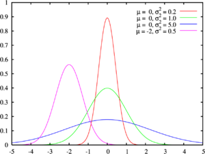
- The normal distribution, also called the Gaussian or the bell curve. It is ubiquitous in nature and statistics due to the central limit theorem: every variable that can be modelled as a sum of many small independent variables is approximately normal.
- The Pearson Type IV distribution (see Pearson distributions)
- Student's t-distribution, useful for estimating unknown means of Gaussian populations.
- The type-1 Gumbel distribution
- The Voigt distribution, or Voigt profile, is the convolution of a normal distribution and a Cauchy distribution. It is found in spectroscopy when spectral line profiles are broadened by a mixture of Lorentzian and Doppler broadening mechanisms.
Joint distributions
For any set of independent random variables the probability density function of their joint distribution is the product of their individual density functions.
Two or more random variables on the same sample space
- Dirichlet distribution, a generalization of the beta distribution.
- The Ewens's sampling formula is a probability distribution on the set of all partitions of an integer n, arising in population genetics.
- Balding-Nichols model
- multinomial distribution, a generalization of the binomial distribution.
- multivariate normal distribution, a generalization of the normal distribution.
Matrix-valued distributions
- Wishart distribution
- matrix normal distribution
- matrix t-distribution
- Hotelling's T-square distribution
Miscellaneous distributions
Demonstrations and activities
The SOCR resource provides web-based tools (applets) for sampling from and interacting with many of these discrete and continuous distributions. Also, a number of distribution-specific activities are provided that demonstrate the utilization of general probability distributions.
See also
- copula (statistics)
- cumulative distribution function
- likelihood function
- list of statistical topics
- probability density function
- histogram
- Inverse transform sampling
- Riemann-Stieltjes integral: Application to probability theory
| |||||||||||||||||||||||||||
| |||||||||||||||||||||||||||
| |||||||||||||||||||||||||||
| |||||||||||||||||||||||||||
| |||||||||||||||||||||||||||
| |||||||||||||||||||||||||||